Data Preprocessing
Import raw microscopy data
Data can be imported from czi and tiff files. The gbeflow.CziImport wraps the czifile module published by Christoph Gohlke to read the propriatory zeiss file format. The underlying datastructure of czi’s varies based on the collection parameters, so the gbeflow.CziImport may not work reliabily.
import gbeflow

# Load czi file from relative/absolute path
czi = gbeflow.CziImport(filepath)

# Raw array of data is available as an attribute
raw = czi.raw_im

# Data squeezed to minimum dimensions also available
data = czi.data
Alternativly, data can be read from tiff files saved using Fiji. The module tifffile makes this by far the easiest approach with tifffile.imread and tifffile.imsave.
import tifffile

# Import tiff file from relative or absolute path
img = tifffile.imread(filepath)

# Save array to new tiff file
tifffile.imsave(outpath, data=img)
Embryo alignment
During imaging, embryos are not expected to be aligned in any particular orientation in the XY plane. While we will accept only embryos that have an approximate lateral mounting, we need to correct XY positioning in post-processing. In the notebook rotate_embryo, a workflow is proposed that accepts user inputs in order to guide the alignment process. The user input functions rely on bebi103 which is a package written by Justin Bois for the BE/Bi103 course that is still under active development. Below is an example of what processing a single sample might look like.
import os
import glob
import tqdm

import numpy as np
import pandas as pd
import scipy.ndimage

import tifffile
import bebi103

import bokeh.io
bokeh.io.output_notebook()

import gbeflow
Import first time point from each original tiff
files = glob.glob(os.path.abspath('../data/original/20181130-gbe_mutants_brt/*.tif'))
files = files
The key parameter for tifffile.imread lets us import just the
first timepoint with both channels. This makes it possible so that we
can look at a sample of all of the data at once. Since the total dataset
is >20Gb we can’t load it directly into memory.
%%time
raw = {}
for f in files:
    raw[f] = tifffile.imread(f,key=(0,1))
Select points to use for alignment
Try selecting two points on the dorsal surface that represent the linear plane of the dorsal side. This approach should hopefully be less sensitive to variability in how the user picks the points.
clicks = []
for f in files:
    clk = bebi103.viz.record_clicks(raw[f][1],flip=False)
    clicks.append(clk)
Extract the points selected for each image into a dataframe.
Ldf = []
for clk in clicks:
    Ldf.append(clk.to_df())

points = pd.concat(Ldf,keys=files)
points
| x | y | ||
|---|---|---|---|
| /Users/morganschwartz/code-block/germband-extension/data/original/20181130-gbe_mutants_brt/20181130-gbe_mutants_brt_05_eve.tif | 0 | 583.782051 | 811.211429 |
| 1 | 819.794872 | 311.188571 | |
| /Users/morganschwartz/code-block/germband-extension/data/original/20181130-gbe_mutants_brt/20181130-gbe_mutants_brt_21_kr.tif | 0 | 182.525641 | 412.960000 |
| 1 | 380.769231 | 829.177143 | |
| /Users/morganschwartz/code-block/germband-extension/data/original/20181130-gbe_mutants_brt/20181130-gbe_mutants_brt_17_kr.tif | 0 | 368.294872 | 650.411429 |
| 1 | 550.384615 | 206.422857 | |
| /Users/morganschwartz/code-block/germband-extension/data/original/20181130-gbe_mutants_brt/20181130-gbe_mutants_brt_23_kr.tif | 0 | 334.474359 | 685.405714 |
| 1 | 352.769231 | 197.600000 |
Reshape points array to have one row per sample.
points = points.reset_index(level=1)
points.head()
| level_1 | x | y | |
|---|---|---|---|
| /Users/morganschwartz/code-block/germband-extension/data/original/20181130-gbe_mutants_brt/20181130-gbe_mutants_brt_05_eve.tif | 0 | 583.782051 | 811.211429 |
| /Users/morganschwartz/code-block/germband-extension/data/original/20181130-gbe_mutants_brt/20181130-gbe_mutants_brt_05_eve.tif | 1 | 819.794872 | 311.188571 |
| /Users/morganschwartz/code-block/germband-extension/data/original/20181130-gbe_mutants_brt/20181130-gbe_mutants_brt_21_kr.tif | 0 | 182.525641 | 412.960000 |
| /Users/morganschwartz/code-block/germband-extension/data/original/20181130-gbe_mutants_brt/20181130-gbe_mutants_brt_21_kr.tif | 1 | 380.769231 | 829.177143 |
| /Users/morganschwartz/code-block/germband-extension/data/original/20181130-gbe_mutants_brt/20181130-gbe_mutants_brt_17_kr.tif | 0 | 368.294872 | 650.411429 |
Calculate a line for each embryo
line = gbeflow.calc_line(points)
line = line.reset_index().rename(columns={'index':'f'})
line.head()
| f | x1 | x2 | y1 | y2 | dx | dy | m | |
|---|---|---|---|---|---|---|---|---|
| 0 | /Users/morganschwartz/code-block/germband-extension/... | 583.782051 | 819.794872 | 811.211429 | 311.188571 | 236.012821 | -500.022857 | -2.118626 |
| 1 | /Users/morganschwartz/code-block/germband-extension/... | 182.525641 | 380.769231 | 412.960000 | 829.177143 | 198.243590 | 416.217143 | 2.099524 |
| 2 | /Users/morganschwartz/code-block/germband-extension/... | 368.294872 | 550.384615 | 650.411429 | 206.422857 | 182.089744 | -443.988571 | -2.438295 |
| 3 | /Users/morganschwartz/code-block/germband-extension/... | 334.474359 | 352.769231 | 685.405714 | 197.600000 | 18.294872 | -487.805714 | -26.663522 |
Plot embryos with line on top
# Create list to collect plot objects
Lp = []

# X values to compute line on
x = np.linspace(0,1024,100)

for f in files:
    p = bebi103.viz.imshow(raw[f][1,:,:],flip=False)

    x1 = line[line['f']==f]['x1'].values
    y1 = line[line['f']==f]['y1'].values
    m = line[line['f']==f]['m'].values
    y = m*(x-x1) + y1

    p.line(x,y,color='red',line_width=3)
#     p.scatter(line[line['f']==f]['x'], line[line['f']==f]['y'],color='white',size=15)

    Lp.append(p)

bokeh.io.show(bokeh.layouts.gridplot(Lp,ncols=2))
Calculate rotation
The angle of rotation is calculated as follows
This calculation can be code-blockd using the np.arctan2, which has two arguments that correspond to \(\Delta y\) and \(\Delta x\).
line = gbeflow.calc_embryo_theta(line)
line.head()
| f | x1 | x2 | y1 | y2 | dx | dy | m | theta | |
|---|---|---|---|---|---|---|---|---|---|
| 0 | /Users/morganschwartz/code-block/germband-extension/... | 583.782051 | 819.794872 | 811.211429 | 311.188571 | 236.012821 | -500.022857 | -2.118626 | -64.732499 |
| 1 | /Users/morganschwartz/code-block/germband-extension/... | 182.525641 | 380.769231 | 412.960000 | 829.177143 | 198.243590 | 416.217143 | 2.099524 | 64.531611 |
| 2 | /Users/morganschwartz/code-block/germband-extension/... | 368.294872 | 550.384615 | 650.411429 | 206.422857 | 182.089744 | -443.988571 | -2.438295 | -67.700358 |
| 3 | /Users/morganschwartz/code-block/germband-extension/... | 334.474359 | 352.769231 | 685.405714 | 197.600000 | 18.294872 | -487.805714 | -26.663522 | -87.852162 |
Apply rotation based on \(\theta\)
With \(\theta\) calculated, we are now ready to rotate each sample accordingly. Since we cannot load all of the data into memory at the same time, we will currently only rotate the first timepoint to check that it worked. After we have determined all necessary manipulations for each embryo, we will run the actual rotation.
# Dataframe to save first timepoint from each rotate embryo
rot = {}

# List to save bokeh plots
Lp = []

for f in tqdm.tqdm(files):
    # Extract the theta value for this sample
    theta = line[line['f']==f]['theta'].values[0]

    # Rotate single image
    rimg = scipy.ndimage.rotate(raw[f][1],theta)

    # Save and plot first timepoint
    rot[f] = rimg
    p = bebi103.viz.imshow(rimg,title=f)
    Lp.append(p)
100%|██████████| 4/4 [00:00<00:00, 6.63it/s]
bokeh.io.show(bokeh.layouts.gridplot(Lp,ncols=2))
# Import modules
import bebi103
import gbeflow
import tifffile
import scipy.ndimage

# Import image from tiff
raw = tifffile.imread(impath)

# Select first timepoint from `raw` to display
clk = bebi103.viz.record_clicks(raw[0],flip=False)

# Extract points from `clk` to a dataframe
points = clk.to_df().reset_index()

# Calculate line for each embryo
line = gbeflow.calc_line(points
                ).reset_index(
                ).rename(
                    columns={'index','f'}
                )

# Calculate angle of rotation
line = gbeflow.calc_embryo_theta(line)

# Rotate embryo
rimg = scipy.ndimage.rotate(raw,line['theta'])

# Save rotated stack to file
tifffile.imsave(outpath,data=rimg)
Manual curation of orientation
After the rotation based on \(\theta\) has been applied, the embryos should be positioned such that the AP axis is horizontal. However, the rotation does not gurantee that the embryo will be positioned with anterior left and dorsal up. At this point, the user can individually specify any additional rotations to correct the embryo’s orientation. The following examples are typically sufficient to correct most orientation errors:
# Rotate by 180 degrees around center point
img = scipy.ndimage.rotate(img,180)

# Flip horizontally by specifying a specific axis
img = np.flip(img,axis=-1)

# Flip vertically
img = np.flip(img,axis=-1)
The final result of this workflow is that all samples are aligned dorsal up with the anterior end of the embryo to the left. This consistent alignment should facilitate future comparisons of the results of optical flow.
Embryo Masking
Rationale
We want to eliminate the background by segmenting the embryo from the background. Later in our analysis, our job will be easier if we do not need to worry about the background contributing noise.
Basic Approach
Segment the embryo from the background in order to clearly isolate changes in signal associated with germ band extension
import numpy as np
import matplotlib.pyplot as plt

from imp import reload
import sys
sys.path.insert(0, '..')
import utilities as ut

from skimage import img_as_float
from skimage.filters import gaussian
from skimage.segmentation import active_contour
from skimage.measure import grid_points_in_poly
Data Import
Read in hdf5 hyperstack as a 3d numpy array. Convert to float for ease of processing.
hst = img_as_float(ut.read_hyperstack('../data/wt_gbe_20180110.h5'))
Select a single image from the first timepoint to use as a test case for segmentation development
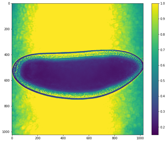
img = hst[0]
ut.imshow(img)
Background Segmentation
In order to analyze any signal variation that is associated with germ band extension, we need to isolate the signal of the embryo from any background. This task is complicated by the nature of brightfield images where the intensity of the background ~1 is similar to the intensity of cells within the image. As a result we cannot use a simple threshold which would remove signal from within the embryo as well as from the background.
However, the embryo does have a clear dark line that separates the embryo itself from the background. We will take advantage of this clear line to separate the embryo from the background using contour based methods.
To start, we will approximate an ellipse that is slightly bigger than the size of the embryo, which will provide a starting point for contour fitting.
# Values to calculate the ellipse over using parametrized trigonometric fxns
s = np.linspace(0, 2*np.pi, 400)

# Define the approximate center of the embryo/ellipse
center_x = 500
center_y = 530

# Define the radius of the ellipse in x and y
radius_x = 550
radius_y = 250

# Calculate the position of the ellipse as a function of s
x = center_x + radius_x*np.cos(s)
y = center_y + radius_y*np.sin(s)
init = np.array([x, y]).T
Next we will use skimage’s active_contour method to fit our
approximated ellipse to the contour of the embryo. The kwarg parameters
for this function were copied based on the active countour
tutorial.
snake = active_contour(gaussian(img, 3),
                       init, alpha=0.015, beta=10, gamma=0.001)
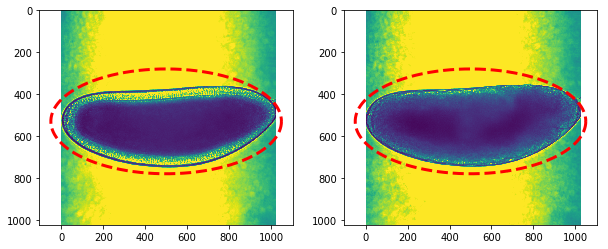
fig,ax = plt.subplots(figsize=(10,10))
ax.imshow(img)
ax.plot(init[:, 0], init[:, 1], '--r', lw=3,label='estimate')
ax.plot(snake[:, 0], snake[:, 1], '-r', lw=3,label='fitted contour')
ax.legend()
<matplotlib.legend.Legend at 0x1c19e6f048>
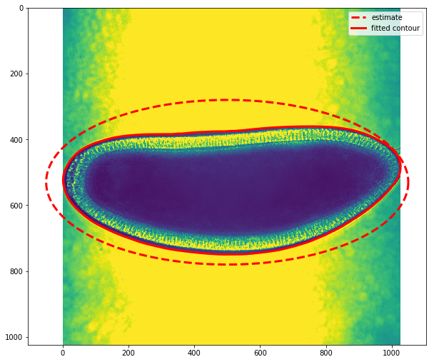
The plot above shows our image overlaid with the approximated ellipse (dashed line) and the fitted counter (red continuous line). This contour follows the boundary between the embryo and the background.
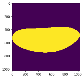
Create background mask
Now that we have a estimated function snake that defines the
boundary of the embryo and the background, we need to define a mask in
the shape of the image that defines which points belong in the image.
Skimage’s grid_points_in_poly function takes a set of points
defining a shape (snake) and identifies which points over a given
raster area fall within the input shape.
mask = grid_points_in_poly(img.shape, snake).T
plt.imshow(mask)
<matplotlib.image.AxesImage at 0x1c1aa11c88>
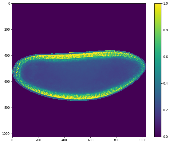
im_masked = img.copy()
im_masked[~mask] = 0
ut.imshow(im_masked)
Write a function to fit a contour to a new embryo
def calc_ellipse(center_x,center_y,radius_x,radius_y):
    '''
    Calculate a parametrized ellipse based on input values
    '''

    # Values to calculate the ellipse over using parametrized trigonometric fxns
    s = np.linspace(0, 2*np.pi, 400)

    # Calculate the position of the ellipse as a function of s
    x = center_x + radius_x*np.cos(s)
    y = center_y + radius_y*np.sin(s)
    init = np.array([x, y]).T

    return(init)
def contour_embryo(img,init):
    '''
    Fit a contour to the embryo to separate the background
    Returns a masked image where all background points = 0
    '''

    # Fit contour based on starting ellipse
    snake = active_contour(gaussian(img, 3),
                       init, alpha=0.015, beta=10, gamma=0.001)

    # Create boolean mask based on contour
    mask = grid_points_in_poly(img.shape, snake).T

    # Apply mask to image and set background to 0
    img[~mask] = 0

    return(img)
Apply mask to hyperstack
Check ellipse approximation on first and last timepoints
center_x,center_y = 500,530
radius_x,radius_y = 550,250
ellipse = calc_ellipse(center_x,center_y,radius_x,radius_y)
fig,ax = plt.subplots(1,2,figsize=(10,8))
ax[0].imshow(hst[0])
ax[0].plot(init[:,0],init[:,1],'--r',lw=3)
ax[1].imshow(hst[-1])
ax[1].plot(init[:,0],init[:,1],'--r',lw=3)
[<matplotlib.lines.Line2D at 0x1c1a65a978>]
# Loop through each timepoint in hyperstack
for t in range(hst.shape[0]):
    hst[t] = contour_embryo(hst[t],ellipse)
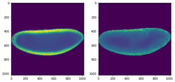
fig,ax = plt.subplots(1,2,figsize=(10,8))
ax[0].imshow(hst[0])
ax[1].imshow(hst[-1])
<matplotlib.image.AxesImage at 0x1c1a3349e8>
Following the development of the method above, an object was created within gbeflow to handle the tasks associated with contouring: MaskEmbryo. An example of using this new class is included below.
import gbeflow
import tifffile
import bebi103

# Import sample from tiff
img = tifffile.imread(filepath)

# Select endpoints of embryo for ellipse calculation
clk = bebi103.viz.record_clicks(raw[0],flip=False)

# Save points to dataframe after selection
points = clk.to_df()

# Initialize object with selected points
me = gbeflow.MaskEmbryo(points)

# Contour embryo based on ellipse calculated during initialization
# Input accepts only 2d data
mask = me.contour_embryo(img[0])

# Apply binary mask to the raw image
mask_img = me.mask_image(img,mask)
After running the code above, this workflow can be applied to the remaining timepoints and saved as a tif.
Limitations
While this approach worked well on the test dataset, when applied to other embryos it would make mistakes on ~10% of frames. There does not appear to be a straightforward way to improve performance without manual curation. See 20181106-endpoint_ellipse.ipynb and 20181108-vector_calculation.ipynb for examples of masking mistakes.
Next Steps
The implementation of contour masking shown in 20181108-vector_calculation.ipynb fits an individual contour to create a mask for each timepoint in the timecourse. Simply by repeating the calculation many times, we introduce more opportunities for mistakes. In the future the contour should be fit just to the first timepoint to create a mask that the optical flow algorithm can use on all timepoints (See the paper’s supplement for more information.) To accommodate any minute changes in embryo size, we could try to increase the size of the mask by 10%, but given the large scale of the movements that we are interested in it may not be necessary.