Simulated Cell Tracking
Objective
While the calculation of the vector field gives us new information about our samples, we still need to develop metrics that enable quantification of the movement of the germband and comparison to other samples. Since there is already an established set of metrics for comparint single cell tracks, we will try to generate single cell tracks from our vector field.
Managing time units
When we run the optical flow algorithm, it takes a parameter for \(\delta t\) however, an initial exploration of the role of this parameter indicates that changing the value does not impact the output of the algorithm. This finding raises the question of what are the units for the vectors output by the algorithm. We will use dimensional analysis of the advection equation to determine the units.
The advection equation describes the movement of a particle carried by a flow
\(\Delta I\) and \(\nabla I\) are defined in arbitrary units (\(\text{au}\)) and describe the change in intensity and the gradient of intensity respectively. The unit of time is not explicitly specified, but we will measure it in seconds (\(\text{s}\)). Given these units, we can calculate the units of \(\mathbf{v}\) (\([\mathbf{v}]\)).
We find that our velociy vector \(\mathbf{v}\) has units of \(1/\text{s}\). When we are calculating the movement of a simulated cell through our fector field, we need to multiply the velocity by the time step in order to calculate the change in position.
Selecting start points
For efficency, we currently ask the user to select a set of points to use as start points for tracks that will be generated using interpolation. We will take advantage of the bebi103 module by using bebi103.viz.record_clicks. In order to record data, the user needs to select the tab on the right side of the figure that shows three points. Then an click on the image will be recorded according to its position.
Interpolation
Currently, the function that interpolates the vector fields for simulated cell tracking gbeflow.VectorField relies on scipy’s interpolate.RectBivariateSpline to estimate the vector for each simulated cell. When gbeflow.VectorField.initialize_interpolation() runs, it saves the scipy interpolation object to gbeflow.VectorField.Ldx or gbeflow.VectorField.Ldy for each timepoint. In order to calculate the trajectory of a single cell, the function gbeflow.VectorField.calc_track() uses the previously calculated interpolation objects stored in gbeflow.VectorField.Ldx and gbeflow.VectorField.Ldy and evaluates the position of the cell to generate the \(x\) and \(y\) components of the next vector.
Code Examples
Data Import
import numpy as np
import pandas as pd
import matplotlib.pyplot as plt

import tifffile

import bebi103

import bokeh.io
# This variable needs to be specified for bokeh to render plots in notebook
notebook_url = 'localhost:8888'
bokeh.io.output_notebook()

import os
import sys
import glob
from imp import reload
import tqdm
import gbeflow
We’ll start by grabbing a list of csv files that were generated by OpticalFlowOutput.m.
csvs = glob.glob('*_Vx.csv')
['yolk3_Vx.csv',
 '20180110_htl_glc_sc6_mmzm_rotate_brt_Vx.csv',
 'yolk_Vx.csv',
 'original_Vx.csv',
 'test3_Vx.csv',
 '20180112_htlglc_tl_sc4_resille_rotate_brt_Vx.csv',
 '20180108_htl_glc_sc2_mmzm_wp_rotate_brt_Vx.csv',
 '20180110_htl_glc-CreateImageSubset-02_sc11_htl_rotate_brt_Vx.csv',
 '20180108_htl_glc_sc9_mmzp_rotate_brt_Vx.csv',
 '20180108_htl_glc_sc11_mmzm_rotate_brt_Vx.csv',
 'test2_Vx.csv',
 '20180112_htlglc_tl_sc11_mmzp_rotate_brt_Vx.csv',
 'test_Vx.csv',
 'yolk2_Vx.csv',
 '20180110_htl_glc_sc15_mmzm_rotate_brt_Vx.csv',
 'sc11_Vx.csv',
 '20180110_htl_glc_sc14_mmzp_rotate_brt_Vx.csv',
 'test4_Vx.csv',
 '20180110_htl_glc-CreateImageSubset-01_sc10_wt_rotate_brt_Vx.csv']
In order to load the data in using gbeflow.tidy_vector_data() we need to isolate the root <name> in the set of file names we collected.
names = set([f[:-7] for f in csvs])
{'20180108_htl_glc_sc11_mmzm_rotate_brt',
 '20180108_htl_glc_sc2_mmzm_wp_rotate_brt',
 '20180108_htl_glc_sc9_mmzp_rotate_brt',
 '20180110_htl_glc-CreateImageSubset-01_sc10_wt_rotate_brt',
 '20180110_htl_glc-CreateImageSubset-02_sc11_htl_rotate_brt',
 '20180110_htl_glc_sc14_mmzp_rotate_brt',
 '20180110_htl_glc_sc15_mmzm_rotate_brt',
 '20180110_htl_glc_sc6_mmzm_rotate_brt',
 '20180112_htlglc_tl_sc11_mmzp_rotate_brt',
 '20180112_htlglc_tl_sc4_resille_rotate_brt',
 'original',
 'sc11',
 'test',
 'test2',
 'test3',
 'test4',
 'yolk',
 'yolk2',
 'yolk3'}
Now we can define a list that just contains the root file names that we are interested in.
fs = ['20180108_htl_glc_sc11_mmzm_rotate_brt',
 '20180108_htl_glc_sc2_mmzm_wp_rotate_brt',
 '20180108_htl_glc_sc9_mmzp_rotate_brt',
 '20180110_htl_glc-CreateImageSubset-01_sc10_wt_rotate_brt',
 '20180110_htl_glc-CreateImageSubset-02_sc11_htl_rotate_brt',
 '20180110_htl_glc_sc14_mmzp_rotate_brt',
 '20180110_htl_glc_sc15_mmzm_rotate_brt',
 '20180110_htl_glc_sc6_mmzm_rotate_brt',
 '20180112_htlglc_tl_sc11_mmzp_rotate_brt',
 '20180112_htlglc_tl_sc4_resille_rotate_brt']
We can now initialize the object gbeflow.VectorField. This object will facilitate importing the data, interpolating over the vector field, and generating simulated cell tracks.
vf = {}
for f in fs:
    vf[f] = gbeflow.VectorField(f)
Each item in the dictionary vf is a vector field object with a key based on the root file name.
vf.keys()
dict_keys(['20180108_htl_glc_sc11_mmzm_rotate_brt',
        '20180108_htl_glc_sc2_mmzm_wp_rotate_brt',
        '20180108_htl_glc_sc9_mmzp_rotate_brt',
        '20180110_htl_glc-CreateImageSubset-01_sc10_wt_rotate_brt',
        '20180110_htl_glc-CreateImageSubset-02_sc11_htl_rotate_brt',
        '20180110_htl_glc_sc14_mmzp_rotate_brt',
        '20180110_htl_glc_sc15_mmzm_rotate_brt',
        '20180110_htl_glc_sc6_mmzm_rotate_brt',
        '20180112_htlglc_tl_sc11_mmzp_rotate_brt',
        '20180112_htlglc_tl_sc4_resille_rotate_brt'])
Now we can import the image data that matches each vector field object.
for f in vf.keys():
    vf[f].add_image_data(os.path.join('../data',vf[f].name+'.tif'))
Track Calculation
Using the image data, we can pick starting points for our tracks. We are going to save the bokeh plotting object generated by gbeflow.VectorField.pick_start_points() into a list so that we can extract the click record when we are done.
L = []
for f in vf.keys():
    L.append(vf[f].pick_start_points())
After points have been selected on each image, we will save the click record back into each vf object.
for i,f in enumerate(vf.keys()):
    vf[f].save_start_points(L[i])
We’re now ready to use interpolation to generate the tracks for each start point.
for f in vf.keys():
    vf[f].calc_track_set(vf[f].starts,60,name='dt60')
Now we can extract the set of tracks from each vf object and save it to a single dataframe for plotting.
# Create a list of track dataframes
Ldf = []
for f in vf.keys():
    Ldf.append(vr[f].tracks)

# Join list of dataframes into a single dataframe
tracks = pd.concat(Ldf,keys=fs)

# Clean up the structure of the dataframe for clarity
tracks = tracks[tracks['name']=='dt60'].reset_index(
                                    ).drop(columns=['level_1']
                                    ).rename(columns={'level_0':'f'})

# Save tracks to csv for later follow up
tracks.to_csv('tracking.csv')
Static Track Visualization
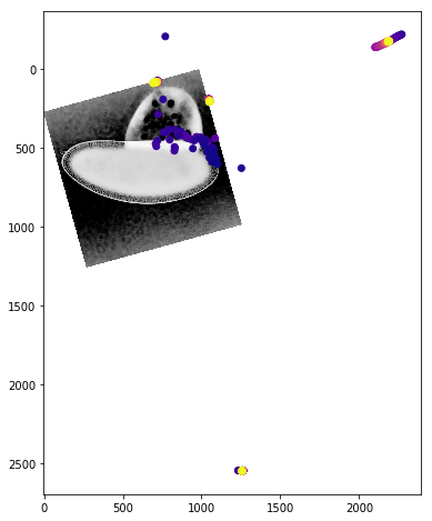
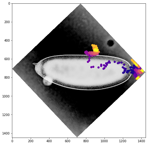
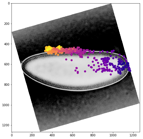
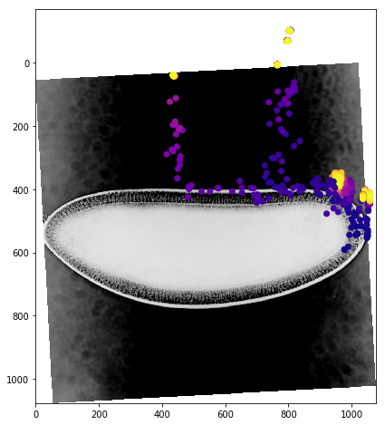
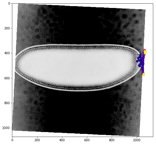
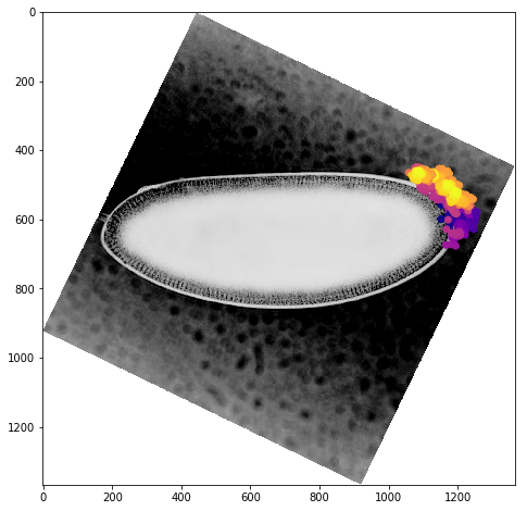
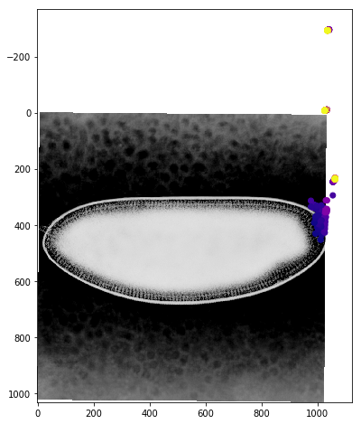
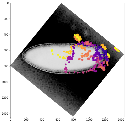
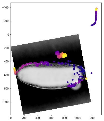
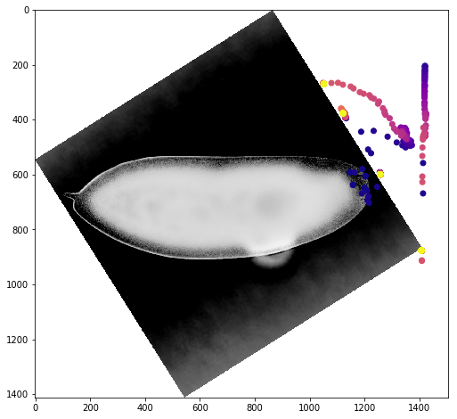
We can get a better sense of the tracking results by plotting the tracks directly on top of the image of the embryo. We’ll look just at the first timepoint and display the image in grey so that we can easily plot on top of it. To show time in our tracks, we’ll color code each point according to its time value using the plasma colormap.
for f in fs:
    fig,ax = plt.subplots(figsize=(10,8))
    ax.imshow(vf.img[0],cmap='Greys')
    sb = tracks[tracks['f']==f]
    ax.scatter(sb.x,sb.y,c=sb['t'].values,cmap='plasma')
Dynamic Track Visualization
In order to get a better sense of how the tracks relate to movement in the embryo, we’ll take advantage of the movie that is automatically generated by OpticalFlowOutput.m. We can read the avi file in as a 3D array using gbeflow.load_avi_as_array(). We can then plot tracks on top of each frame from the avi using gbeflow.make_track_movie(). This second functions saves the new 3D array as a tiff stack, which can be opened in Fiji and converted to an avi if necessary.
for f in fs:
    try:
        gbeflow.make_track_movie(f+'.avi',
                                tracks[tracks.f==f],
                                c='r',
                                name=f+'_tracks')
    except:
        print('Failed:',f)
The python framework of try except is convenient here because the avi output from OpticalFlowOutput.m does not always work and can result in the creation of a file without any data. By using try except, we will get a report if any particular file fails, but our loop will continue running to finish the remaining files.